Differing OAS models rarely return the same Effective Duration numbers. Why is that so? There are a number of reasons why these numbers will not match. One of the chief reasons is that each model is different – some are log-normal, some are Black-Derman-Toy, etc. In addition, most models take shortcuts in order to speed up processing of what can be millions of calculations on a portfolio of a few hundred bonds. Then there are differences to the inputs. The yield curve used, the size of the basis point interval used, and volatility inputs will all affect the output produced by the same model. However, in most cases the single most important factor affecting Effective Duration will be the volatility input chosen. The higher the volatility used, the greater the range of possible future values for each bond at future dates. As this produces both higher and lower future rates, more calls will be in-the-money for the lower rates and more will be out-of-the-money for the higher rates. These calls going in and out of the money have the largest effect on Effective Duration.
Selection of a Volatility Setting
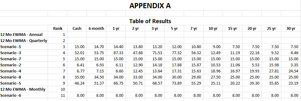
Since volatility is likely to be the single most important factor affecting Effective Duration the logical next question should be “What is the right volatility setting to use?” There are a variety of common answers to this question including: the implied volatility of current options, a single long-term historical volatility for the asset class and the historical volatility of key rates for the asset class. While there are theoretical answers for each of these a more pragmatic approach would argue that the ideal volatility is the one that produces Effective Duration numbers that best correlate to the actual responsiveness of securities to interest rate moves. At Investortools we took that approach to the Effective Duration of municipal bonds. Using ten years’ worth of monthly historical data on over 50,000 bonds and a variety of volatility settings, we compared each bond’s price movement to what would be expected from its Effective Duration and the actual change in the corresponding yield curve point for the month. ( See Appendix A for details.)
Generally, the results showed that lower volatility settings fit the data best for the first three years (2005 through 2007) and higher volatility settings produced the best fit and for the next four years (2008 through 2011). The pattern was less clear after that. None of this should have been a surprise to even a casual observer of fixed income markets during the time. Since all of these tests were run using each possible volatility settings for the entire ten year period, the next step was to use market information that would have been available at the time to compute dynamic volatility settings that reflected contemporary market conditions. The best results were obtained using an exponentially-weighted moving average of the forward spot rates for eleven key rate points. Finally, we asked how frequently should the settings be re-computed? From looking at the data over the entire period, it was obvious that too frequent updates of the volatility assumptions could lead to whipsawing effect, but infrequent updates would lead to stale volatilities that took too long to reflect significant changes in market conditions, especially structural changes like we saw in the last part of 2008. We compared monthly, quarterly and annual updates and determined that annual update frequency was optimal, while quarterly was a close second. Monthly updates produced very poor fits as the whipsawing effect was indeed present. It is therefore our opinion that the best estimate of Effective Duration will be obtained by using an historical weighted average of forward spot rates at key points on the curve, using a one year look back period and that this number should be updated annually. One caveat would be that a practitioner should feel free to override these settings if and when a substantial structural change has occurred, as it did with the Lehman collapse in September of 2008.
How Error Was Calculated
The expected price change for each bond in each volatility scenario was defined as the product of its computed Effective Duration times the change in yield at the point on the yield curve corresponding to the bond’s maturity.
Expected change = -Di x (Y2-Y1)
The actual price change was computed for each bond as the difference between the bond’s actual ending price and a theoretical ending price if the bond were still priced at its beginning yield; divided by the bond’s beginning price. (All prices include accrued interest.)
Actual = (P2 – P’) / P1
The error was defined as the absolute value of the difference between the expected and actual price changes.
Error = ABS(Expected – Actual)
Di = Effective Duration produced by Volatility Scenario i
Y1 = Yield Curve value at start of month
Y2 = Yield Curve value at end of month
P1 = Price at start of month, including accrued interest
P2 = Price at end of month, including accrued interest
P’ = Price of bond at end of month computed using Y1, including accrued interest
Stuart Graydon Jr.
Chairman
Investortools